

Overview
Backpropagation algorithm is probably the most fundamental building block in a neural network. It was first introduced in 1960s and almost 30 years later (1989) popularized by Rumelhart, Hinton and Williams in a paper called "Learning representations by back-propagating errors".
The algorithm is used to effectively train a neural network through a method called chain rule. In simple terms, after each forward pass through a network, backpropagation performs a backward pass while adjusting the model’s parameters (weights and biases).
Define the neural network model
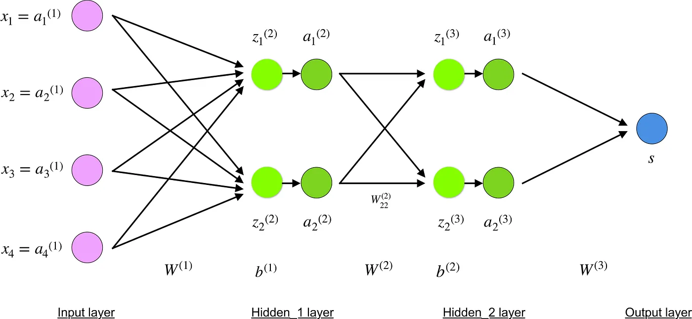
The 4-layer neural network consists of 4 neurons for the input layer, 4 neurons for the hidden layers and 1 neuron for the output layer.
Input layer
The neurons, colored in purple, represent the input data. These can be as simple as scalars or more complex like vectors or multidimensional matrices.
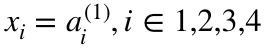
The first set of activations (a) are equal to the input values. NB: “activation” is the neuron’s value after applying an activation function. See below.
Hidden layers
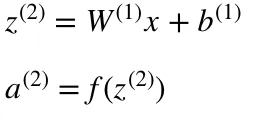
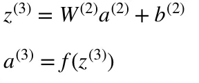
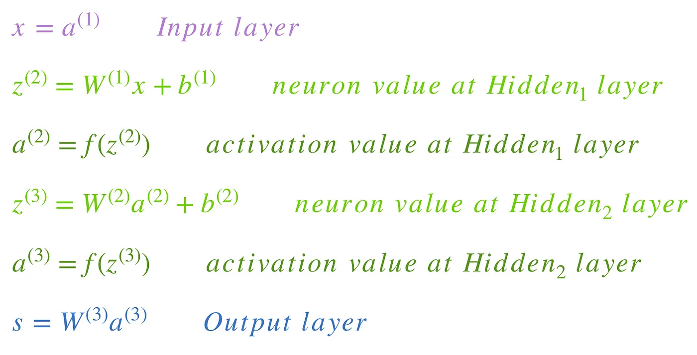
The final values at the hidden neurons, colored in green, are computed using z^l — weighted inputs in layer l, and a^l— activations in layer l. For layer 2 and 3 the equations are:
- l = 2
- l = 3
W² and W³ are the weights in layer 2 and 3 while b² and b³ are the biases in those layers.
Activations a² and a³ are computed using an activation function f. Typically, this function f is non-linear (e.g. sigmoid, ReLU, tanh) and allows the network to learn complex patterns in data. We won’t go over the details of how activation functions work, but, if interested, I strongly recommend reading this great article.
Looking carefully, you can see that all of x, z², a², z³, a³, W¹, W², b¹ and b² are missing their subscripts presented in the 4-layer network illustration above. The reason is that we have combined all parameter values in matrices, grouped by layers. This is the standard way of working with neural networks and one should be comfortable with the calculations. However, I will go over the equations to clear out any confusion.
Let’s pick layer 2 and its parameters as an example. The same operations can be applied to any layer in the network.
- W¹ is a weight matrix of shape (n, m) where n is the number of output neurons (neurons in the next layer) and m is the number of input neurons (neurons in the previous layer). For us, n = 2 and m = 4.
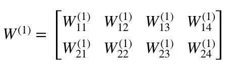
NB: The first number in any weight’s subscript matches the index of the neuron in the next layer (in our case this is the Hidden_2 layer) and the second number matches the index of the neuron in previous layer (in our case this is the Input layer).
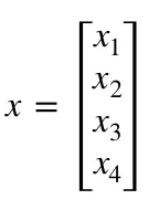
- x is the input vector of shape (m, 1) where m is the number of input neurons. For us, m = 4.
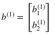
- b¹ is a bias vector of shape (n , 1) where n is the number of neurons in the current layer. For us, n = 2.
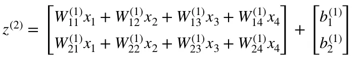
- Following the equation for z², we can use the above definitions of W¹, x and b¹ to derive “Equation for z²”:
Now carefully observe the neural network illustration from above.
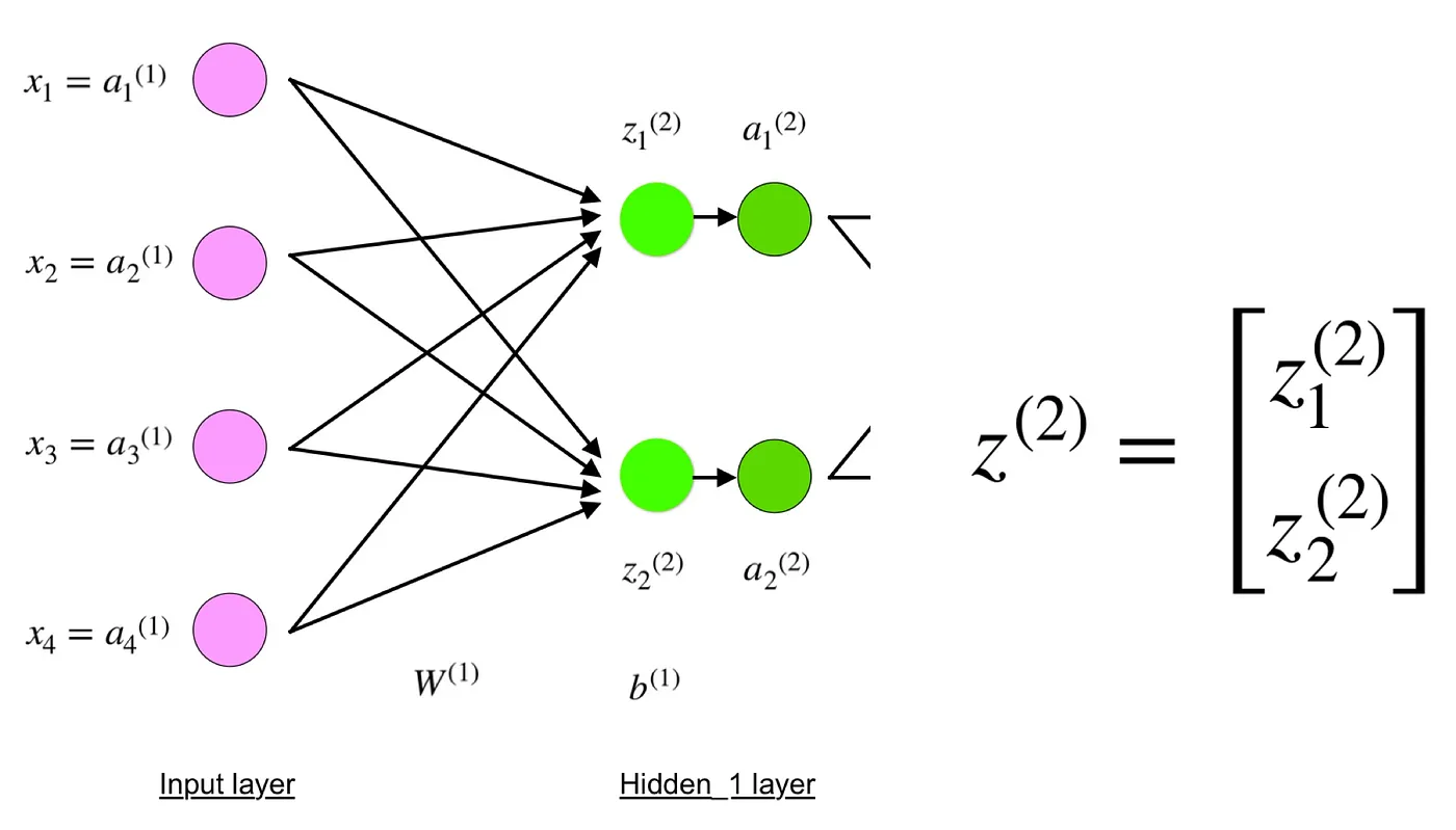
You will see that z² can be expressed using (z_1)² and (z_2)² where (z_1)² and (z_2)² are the sums of the multiplication between every input x_i with the corresponding weight (W_ij)¹.
This leads to the same “Equation for z²” and proofs that the matrix representations for z², a², z³ and a³ are correct.
Output layer
The final part of a neural network is the output layer which produces the predicated value. In our simple example, it is presented as a single neuron, colored in blue and evaluated as follows:
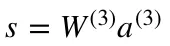
Again, we are using the matrix representation to simplify the equation. One can use the above techniques to understand the underlying logic.
Forward propagation and evaluation
The equations above form network’s forward propagation. Here is a short overview:
The final step in a forward pass is to evaluate the predicted output s against an expected output y.
The output y is part of the training dataset (x, y) where x is the input (as we saw in the previous section).
Evaluation between s and y happens through a cost function. This can be as simple as MSE (mean squared error) or more complex like cross-entropy.
We name this cost function C and denote it as follows:
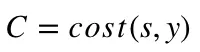
were cost can be equal to MSE, cross-entropy or any other cost function.
Based on C’s value, the model “knows” how much to adjust its parameters in order to get closer to the expected output y. This happens using the backpropagation algorithm.
Backpropagation and computing gradients
According to the paper from 1989, backpropagation:
repeatedly adjusts the weights of the connections in the network so as to minimize a measure of the difference between the actual output vector of the net and the desired output vector.
and
the ability to create useful new features distinguishes back-propagation from earlier, simpler methods…
In other words, backpropagation aims to minimize the cost function by adjusting network’s weights and biases. The level of adjustment is determined by the gradients of the cost function with respect to those parameters.
One question may arise — why computing gradients?
To answer this, we first need to revisit some calculus terminology:
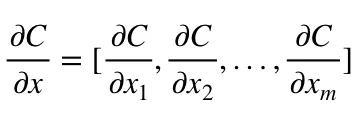
- Gradient of a function C(x_1, x_2, …, x_m) in point x is a vector of the partial derivatives of C in x.
-
The derivative of a function C measures the sensitivity to change of the function value (output value) with respect to a change in its argument x (input value). In other words, the derivative tells us the direction C is going.
-
The gradient shows how much the parameter x needs to change (in positive or negative direction) to minimize C.
Compute those gradients happens using a technique called chain rule.
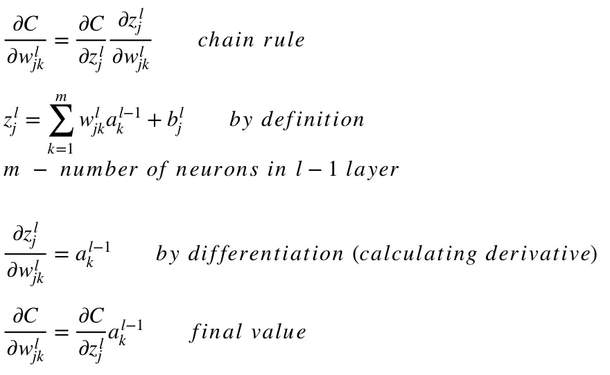
For a single weight (w_jk)^l, the gradient is:
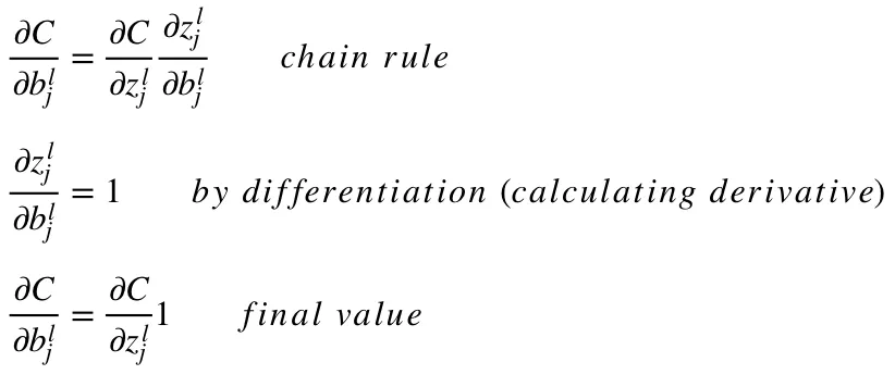
Similar set of equations can be applied to (b_j)^l:
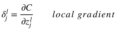
The common part in both equations is often called “local gradient” and is expressed as follows:
The “local gradient” can easily be determined using the chain rule. I won’t go over the process now but if you have any questions, please comment below.
The gradients allow us to optimize the model’s parameters:
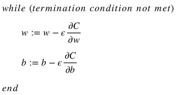
- Initial values of w and b are randomly chosen.
- Epsilon (e) is the learning rate. It determines the gradient’s influence.
- w and b are matrix representations of the weights and biases. Derivative of C in w or b can be calculated using partial derivatives of C in the individual weights or biases.
- Termination condition is met once the cost function is minimized.
I would like to dedicate the final part of this section to a simple example in which we will calculate the gradient of C with respect to a single weight (w_22)².
Let’s zoom in on the bottom part of the above neural network:
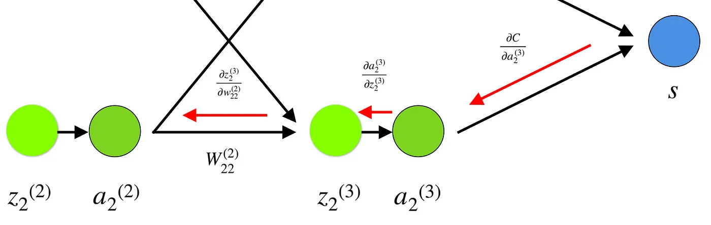
Weight (w_22)² connects (a_2)² and (z_2)², so computing the gradient requires applying the chain rule through (z_2)³ and (a_2)³:
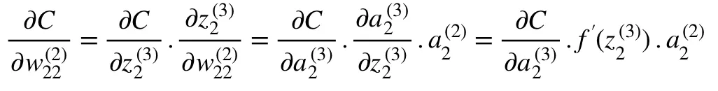
Calculating the final value of derivative of C in (a_2)³ requires knowledge of the function C. Since C is dependent on (a_2)³, calculating the derivative should be fairly straightforward.
I hope this example manages to throw some light on the mathematics behind computing gradients. To further enhance your skills, I strongly recommend watching Stanford’s NLP series where Richard Socher gives 4 great explanations of backpropagation.