Linear Algebra explained in the context of deep learning

Linear algebra is the branch of mathematics concerning linear equations and linear functions and their representations through matrices and vector spaces. (Wikipedia)

Introduction

If you start to learn deep learning , the first thing you will be exposed to is the feed forward neural network, which is the most simple and also highly useful network in deep learning. Under the hood, the feed forward neural network is just a composite function, that multiplies some matrices and vectors together.

It is not that vectors and matrices are the only way to do these operations but they become highly efficient if you do so.

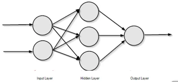
The image above shows a simple feed forward neural network that propagates information forwards.

The image is a beautiful representation of the neural network, but how a computer can understand this. In a computer, the layers of the neural network are represented as vectors. Consider the input layer as X and the hidden layer as H. The output layer is not concerned for now.(The computation process of feed forward neural networks is not concerned here.)

So, it can be represented as a vectors and matrices as

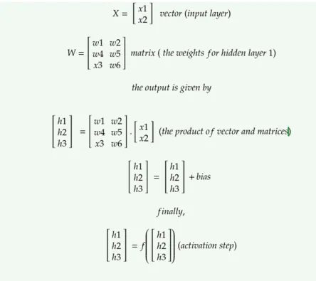
The above image shows the operations needed to compute the output for the first and the only hidden layer of the above neural network(the computation for the output layer is not shown). Let’s break it down.

Every single column of the network are vectors.Vectors are dynamic arrays that are a collection of data(or features).In the current neural network, the vector ‘x’ holds the input.It is not mandatory to represent inputs as vectors but if you do so, they become increasingly convenient to perform operations in parallel.

Mathematical perspective of Vectors and matrices

Deep learning and in specific, neural networks are computationally expensive, so they require this nice trick to make them compute faster.

It’s called vectorization. They make computations extremely faster.This is one of the main reasons why GPUs are required for deep learning, as they are specialized in vectorized operations like matrix multiplication.(we’ll see this in the end in depth).

The hidden layer H’s output is calculated by performing H = f( W.x + b ).

Here W is called as the Weight matrix, b is called bias and f is the activation function.(this article does not explain about feed forward neural networks, if you need a primer about the concept of FFNN, look here.)

Let’s breakdown the equation,

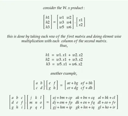
the first component is W.x ; this is a matrix-vector product, because W is a matrix and x is a vector.Before getting into multiplying these, let’s get some idea about the notations: usually vectors are denoted by small bold italic letters(like x) and matrices are denoted by capital bold italic letters(like X).If the letter is capital and bold but not italic then it is a tensor(like X).

In a computer science perspective

• Scalar: A single number.
• Vector : A list of values.(rank 1 tensor)
• Matrix: A two dimensional list of values.(rank 2 tensor)
• Tensor: A multi dimensional matrix with rank n.

Drilling down:

In a mathematical perspective

Vector

A vector is a quantity that has both magnitude and direction.It is an entity that exists in space, it’s existence is denoted by x∈ ℝ²if it is a 2 dimensional vector that exists in real space.(Each element denotes a coordinate along a different axis.)

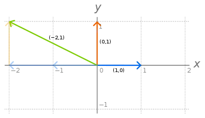
All vectors in 2D space can be obtained by linear combination of the two vectors called basis vectors.( denoted by i and j ) (In general, a vector in N dimensions can be represented by N basis vectors.). They are unit normal vectors because their magnitude is one and they are perpendicular to each other. One of these two vectors can’t be represented by the other vector. So they are called as linearly independent vectors. (If any vector can’t be obtained by a linear combination of a set of vectors, then the vector is linearly independent from that set). All the set of points in the 2D space that can be obtained by linear combination of these two vectors are said to be the span of these vectors.If a vector is represented by a linear combination (addition, multiplication) of set of other vectors, then it is linearly dependent on that set of vectors.(there is no use in adding this new vector to the existing set.)

Any two vectors can be added together.They can be multiplied together.Their multiplication is of two types, dot product and cross product. Refer here.

Matrix

A matrix is a 2D array of numbers. They represent transformations. Each column of a 2x2 matrix denotes each of the 2 basis vectors after the 2D space is applied with that transformation.Their space representation is W ∈ ℝ³*² having 3 rows and 2 columns.

A matrix vector product is called transformation of that vector, while a matrix matrix product is called as composition of transformations.

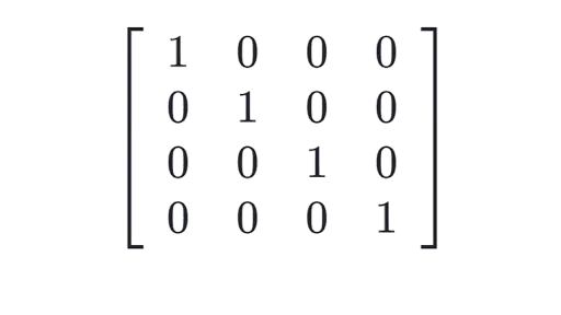
There is only one matrix which does not does any transformation to the vector.It is the identity matrix(I). The columns of I represent the basis vectors.

Determinant of the matrix A, denoted by det(A) the the scaling factor of the linear transformation described by the matrix.

Why is a mathematical perspective important to deep learning researchers? Because they help us understand the basic design concepts of fundamental objects.They also help in crafting creative solutions to a deep learning problems. But no worries, there are a lot of languages and packages that do these implementations for us. But it’s also good to know their implementations.

One such library is numpy for python programming language.

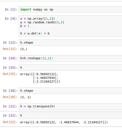
There are lots of resources for learning numpy.(which is very important for learning deep learning, if you use python.) look here.

Here, np.array creates a numpy array.

np.random is a package that contains methods for random number generation.

the dot method is to compute product between matrix.

We can change the shape of the numpy array and also check it.

here you can see that, the product of W.x is a vector and it is added with b, which is a scalar. This automatically expands b as transpose([1,1]). This implicit copying of b to several locations is called as broadcasting. (we’ll see in depth in a moment.)

Did you notice the word transpose: The transpose of a matrix is a mirror image of the matrix across the diagonal line(from top left to the bottom right of the matrix.)

1## numpy code for transpose
2import numpy as np
3A = np.array([[1,2],
4              [3,4],
5              [5,6]])
6B = np.transpose(A) 
7##or
8B = A.T

Types of matrices

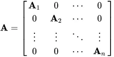
Diagonal matrix: All the elements are zero except the main diagonal elements.

Identity matrix: a diagonal matrix with diagonal values as 1.

1## numpy code to create identity matrix
2import numpy as np
3a = np.eye(4)

Symmetric matrix: A matrix which is equal to it’s transpose. A = transpose(A)

Singular matrix: a matrix whose determinant is zero and columns are linearly dependent.Their rank is less than the number of rows or columns of the matrix.

Decomposition of matrices:

A matrix decomposition or matrix factorization is a factorization of a matrix into a product of matrices. There are many different matrix decompositions; each finds use among a particular class of problems.One of the most widely used kinds of matrix decomposition is called eigen decomposition, in which we decompose a matrix into a set of eigenvectors and eigenvalues.

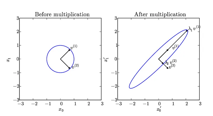
An Eigen vector of a square matrix A is a non zero vector v such that multiplication by A alters only the scale of v.

A . v = lambda . v

Here v is the eigen vector and lambda is the eigen value.

1## numpy program to find eigen vectors.
2
3from numpy import array
4from numpy.linalg import eig
5# define matrix
6A = array([[1, 2, 3], [4, 5, 6], [7, 8, 9]])
7print(A)
8# calculate eigendecomposition
9values, vectors = eig(A)
10print(values)
11print(vectors)

Eigen decomposition is very useful in machine learning. It is particularly useful for concepts like dimensionality reduction.

For more about eigen decomposition, refer deep learning book, chapter 2

There are also several other matrix decomposition techniques used in deep learning. Look here.

Norms

Overfitting and underfitting

When you attend a deep learning lecture, you often hear the term overfitting and underfitting.These terms describe the state of the accuracy of the deep learning model.

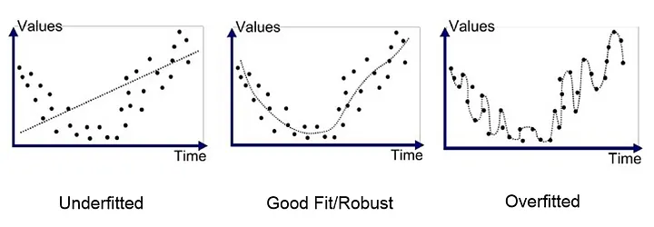
Overfitting refers to a model that learns the training data too well.It literally mugged up the training data.In overfit models, the training accuracy is very high and validation accuracy is very low.

Underfit models have not managed to learn the training data.In underfit models, the training and validation accuracy are both very low.

Both overfitting and underfitting can lead to poor model performance. But by far the most common problem in applied machine learning is overfitting.

To reduce overfitting, we have to use a technique called Regularization. It prevents mugging up the training data, so as to avoid the risk of overfitting.

It is the most important responsibility of the deep learning engineer to create a model which fits generally to the input. There are several methods of regularization.Most notably the L1 regularization( Lasso ) and L2 regularization( Ridge ).

The details of these are not provided, but to understand these you must know what is a norm.

Norm

Norm is the size of the vector.The general formula for norm of a vector x is given by

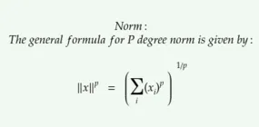
the L² norm with p=2 is called the euclidean norm because it is the euclidean distance between origin and x.

The L¹ norm is simply the sum of all the elements of the vector.It is used in machine learning when the system requires much more precision.To differentiate clearly between a zero and a non zero element. The L¹ norm is also known as Manhattan norm.

There is also max norm, which is the absolute value of the element with the largest magnitude.

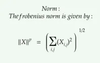
The L² norm equivalent for a matrix is the frobenius norm.

Not only in regularization, norms are used also in optimization procedures.

Ok, now after all these concepts and theory, we have come to cover the most important part required for deep learning.They are vectorization and broadcasting.

Vectorization

It is the trick of reducing execution of loops and make process execute in parallel by providing data as vectors.

Many CPUs have “vector” or “SIMD”(Single Instruction Multiple Data) instruction sets which apply the same operation simultaneously to two, four, or more pieces of data. SIMD became popular on general-purpose CPUs in the early 1990s.

For more detailed information, look for Flynn’s classification.

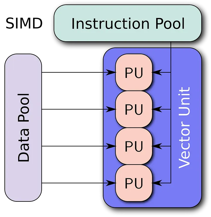
Vectorization is the process of rewriting a loop so that instead of processing a single element of an array N times, it processes (say) 4 elements of the array simultaneously N/4 times.

Numpy has heavily implemented vectorization into their algorithms. Here is an official note from numpy.

Vectorization describes the absence of any explicit looping, indexing, etc., in the code — these things are taking place, of course, just “behind the scenes” in optimized, pre-compiled C code. Vectorized code has many advantages, among which are:

vectorized code is more concise and easier to read

fewer lines of code generally means fewer bugs

the code more closely resembles standard mathematical notation (making it easier, typically, to correctly code mathematical constructs)

vectorization results in more “Pythonic” code. Without vectorization, our code would be littered with inefficient and difficult to read for loops.

Code example:

1## to add two arrays together.
2## consider two basic python lists.
3a = [1,2,3,4,5]
4b = [2,3,4,5,6]
5c = []
6## without vectorization.
7for i in range(len(a)): 
8    c.append(a[i]+b[i])
9## using vectorization.
10a = np.array([1,2,3,4,5])
11b = np.array([2,3,4,5,6])
12c = a+b

The above code example is an overly simplified example of vectorization. And vectorization really comes into picture when the input data becomes large.

For more details about vectorization, look here.

Broadcasting

The next important concept is broadcasting. Sir Jeremy Howard in one of his machine learning lectures, told that broadcasting is probably the most important tool and a skill to have for a machine learning programmer.

From the Numpy Documentation:

The term broadcasting describes how numpy treats arrays with different shapes during arithmetic operations. Subject to certain constraints, the smaller array is “broadcast” across the larger array so that they have compatible shapes. Broadcasting provides a means of vectorizing array operations so that looping occurs in C instead of Python. It does this without making needless copies of data and usually leads to efficient algorithm implementations.

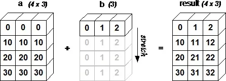
Code example:

1a = np.array([1.0, 2.0, 3.0])
2b = 2.0
3a * b
4array([ 2.,  4.,  6.])
5
6# this is similar to
7
8a = np.array([1.0, 2.0, 3.0])
9b = np.array([2.0, 2.0, 2.0])
10a * b
11array([ 2.,  4.,  6.])

The array b is expanded so that arithmetic operation can be applied.

Broadcasting is not a new concept. It is a relative old tool that dates back to 50’s. In his paper “Notation as a tool of thought”, Kenneth Iverson describes several tools for mathematical usage that allows us to think in new perspectives. Broadcasting was first mentioned by him not as a computer algorithm but as a mathematical procedure.He implemented many of these tools in a software called APL.

His son later extended his ideas and went on to create another software called J software. This gesture means that with software what we get is over 50 years of deep research and using these we can implement very complex mathematical functions in a small piece of code.

It is also very handy that these researches have also found their way into languages we use today like python and numpy.

So bear in mind that these are not very simple ideas that came overnight. These are like the fundamental ways to think of mathematics and it’s implementation in software. (The above content is extracted from fast.ai machine learning course.)

For more details about numpy version of broadcasting, look here.

References

• 3Blue1Brown Linear Algebra Series
• Ebook
• Site to learn deep learning
• A complete learning book
• Article on linear algebra