What is a Vector Database?
A vector database indexes and stores vector embeddings for fast retrieval and similarity search, with capabilities like CRUD operations, metadata filtering, horizontal scaling, and serverless.
We’re in the midst of the AI revolution. It’s upending any industry it touches, promising great innovations - but it also introduces new challenges. Efficient data processing has become more crucial than ever for applications that involve large language models, generative AI, and semantic search.
All of these new applications rely on vector embeddings, a type of vector data representation that carries within it semantic information that’s critical for the AI to gain understanding and maintain a long-term memory they can draw upon when executing complex tasks.
Embeddings are generated by AI models (such as Large Language Models) and have many attributes or features, making their representation challenging to manage. In the context of AI and machine learning, these features represent different dimensions of the data that are essential for understanding patterns, relationships, and underlying structures.
That is why we need a specialized database designed specifically for handling this data type. Vector databases like Pinecone fulfill this requirement by offering optimized storage and querying capabilities for embeddings. Vector databases have the capabilities of a traditional database that are absent in standalone vector indexes and the specialization of dealing with vector embeddings, which traditional scalar-based databases lack.
The challenge of working with vector data is that traditional scalar-based databases can’t keep up with the complexity and scale of such data, making it difficult to extract insights and perform real-time analysis. That’s where vector databases come into play – they are intentionally designed to handle this type of data and offer the performance, scalability, and flexibility you need to make the most out of your data.
We are seeing the next generation of vector databases introduce more sophisticated architectures to handle the efficient cost and scaling of intelligence. This ability is handled by serverless vector databases, that can separate the cost of storage and compute to enable low-cost knowledge support for AI.
With a vector database, we can add knowledge to our AIs, like semantic information retrieval, long-term memory, and more. The diagram below gives us a better understanding of the role of vector databases in this type of application:
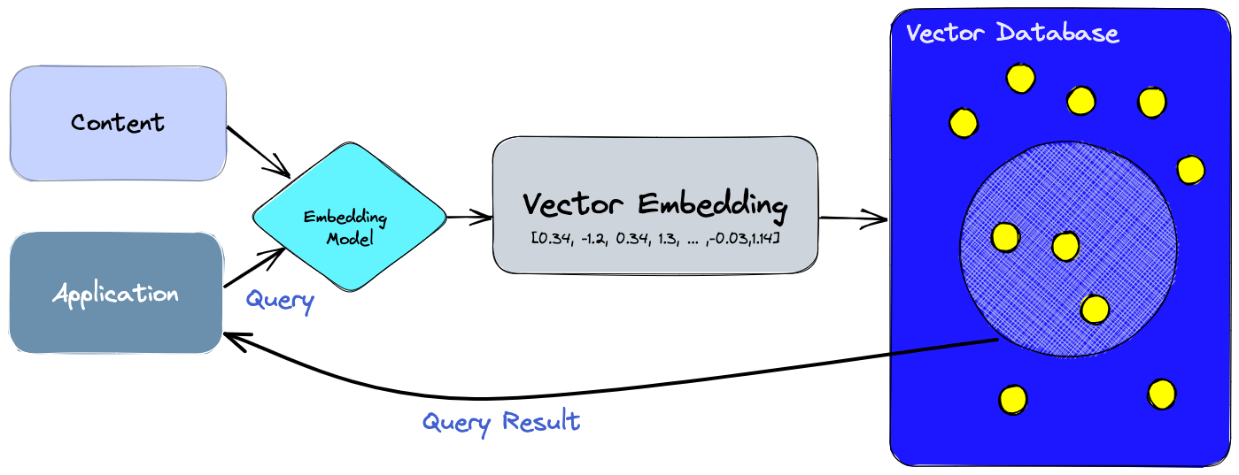
Let’s break this down:
-
First, we use the embedding model to create vector embeddings for the content we want to index.
-
The vector embedding is inserted into the vector database, with some reference to the original content the embedding was created from.
-
When the application issues a query, we use the same embedding model to create embeddings for the query and use those embeddings to query the database for similar vector embeddings. As mentioned before, those similar embeddings are associated with the original content that was used to create them.
What's difference between a vector index and a vector database?
Standalone vector indices like FAISS (Facebook AI Similarity Search) can significantly improve the search and retrieval of vector embeddings, but they lack capabilities that exist in any database. Vector databases, on the other hand, are purpose-built to manage vector embeddings, providing several advantages over using standalone vector indices:
-
Data management: Vector databases offer well-known and easy-to-use features for data storage, like inserting, deleting, and updating data. This makes managing and maintaining vector data easier than using a standalone vector index like FAISS, which requires additional work to integrate with a storage solution.
-
Metadata storage and filtering: Vector databases can store metadata associated with each vector entry. Users can then query the database using additional metadata filters for finer-grained queries.
-
Scalability: Vector databases are designed to scale with growing data volumes and user demands, providing better support for distributed and parallel processing. Standalone vector indices may require custom solutions to achieve similar levels of scalability (such as deploying and managing them on Kubernetes clusters or other similar systems). Modern vector databases also use serverless architectures to optimize cost at scale.
-
Real-time updates: Vector databases often support real-time data updates, allowing for dynamic changes to the data to keep results fresh, whereas standalone vector indexes may require a full re-indexing process to incorporate new data, which can be time-consuming and computationally expensive. Advanced vector databases can use performance upgrades available via index rebuilds while maintaining freshness.
-
Backups and collections: Vector databases handle the routine operation of backing up all the data stored in the database. Pinecone also allows users to selectively choose specific indexes that can be backed up in the form of “collections,” which store the data in that index for later use.
-
Ecosystem integration: Vector databases can more easily integrate with other components of a data processing ecosystem, such as ETL pipelines (like Spark), analytics tools (like Tableau and Segment), and visualization platforms (like Grafana) – streamlining the data management workflow. It also enables easy integration with other AI related tooling like LangChain, LlamaIndex, Cohere, and many others..
-
Data security and access control: Vector databases typically offer built-in data security features and access control mechanisms to protect sensitive information, which may not be available in standalone vector index solutions. Multitenancy through namespaces allows users to partition their indexes fully and even create fully isolated partitions within their own index.
In short, a vector database provides a superior solution for handling vector embeddings by addressing the limitations of standalone vector indices, such as scalability challenges, cumbersome integration processes, and the absence of real-time updates and built-in security measures, ensuring a more effective and streamlined data management experience.
How does a vector database work?
We all know how traditional databases work (more or less)—they store strings, numbers, and other types of scalar data in rows and columns. On the other hand, a vector database operates on vectors, so the way it’s optimized and queried is quite different.
In traditional databases, we are usually querying for rows in the database where the value usually exactly matches our query. In vector databases, we apply a similarity metric to find a vector that is the most similar to our query.
A vector database uses a combination of different algorithms that all participate in Approximate Nearest Neighbor (ANN) search. These algorithms optimize the search through hashing, quantization, or graph-based search.
These algorithms are assembled into a pipeline that provides fast and accurate retrieval of the neighbors of a queried vector. Since the vector database provides approximate results, the main trade-offs we consider are between accuracy and speed. The more accurate the result, the slower the query will be. However, a good system can provide ultra-fast search with near-perfect accuracy.
Here’s a common pipeline for a vector database:

-
Indexing: The vector database indexes vectors using an algorithm such as PQ, LSH, or HNSW (more on these below). This step maps the vectors to a data structure that will enable faster searching.
-
Querying: The vector database compares the indexed query vector to the indexed vectors in the dataset to find the nearest neighbors (applying a similarity metric used by that index)
-
Post Processing: In some cases, the vector database retrieves the final nearest neighbors from the dataset and post-processes them to return the final results. This step can include re-ranking the nearest neighbors using a different similarity measure.
Serverless Vector Databases
Serverless represents the next evolution of vector databases. The above architectures get us to a vector database architecture that is accurate, fast, scalable, but expensive. This architecture is what we see in first-generation vector DBs. With the rise of AI use cases where cost and elasticity are increasingly important, a second generation of serverless vector databases is needed.
First-generation vector DBs have three critical pain points that a serverless vector database solves:
-
Separation of storage from compute: To optimize costs, compute should only be used when needed. That means decoupling the index storage from queries and searching only what is needed — this becomes increasingly difficult when involving latency.
-
Multitenancy: Handling namespaces in indexes to ensure infrequently queried namespaces do not increase costs.
-
Freshness: A vector DB needs to provide fresh data, meaning within a few seconds of inserting new data, it is queryable. Note, for Pinecone Serverless freshness can be delayed when inserting large amounts of data.
To separate storage from compute highly sophisticated geometric partitioning algorithms can break an index into sub-indices, allowing us to focus the search on specific partitions:
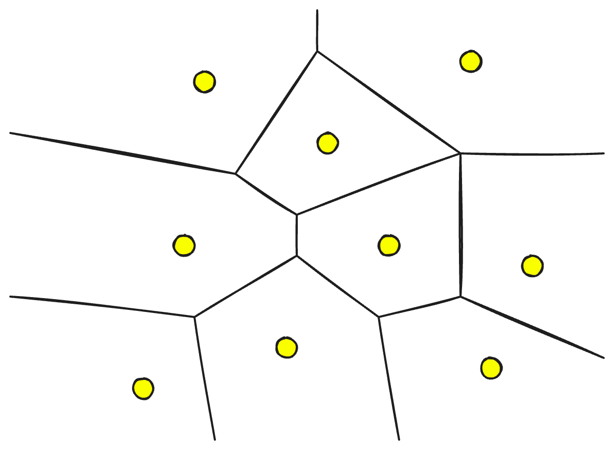
With these partitions, the search space of a query can focus on just a few parts of a vector index rather than the full search space. Typical search behaviors will show that certain partitions are accessed more frequently than others, allowing us to dial between compute costs and cold startup times to find an optimal balance between cost and latency.
When we do this partitioning, we solve the separation of compute and storage problem. However, geometric partitioning is a slower process at index build time. Meaning we can run into freshness problems as we must wait for new data to be correctly stored in the index.
To solve this problem, a vector database needs another separate layer called a freshness layer. The freshness layer acts as a temporary “cache” of vectors that can be queried. At the same time, we wait for an index builder to place new vectors into the geometrically partitioned index.
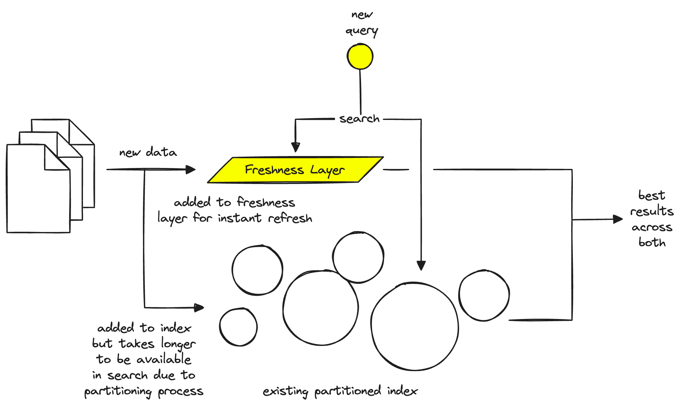
During this process, a query router can send queries to both the index and the freshness layer — solving the freshness problem. However, it’s worth noting that the freshness layer exists in compute instances, so we cannot store the full index there. Instead, we wait for the new vectors to be inserted into the index — once complete, they are removed from the freshness layer.
Finally, there is the problem of multi tenancy. Many first-generation vector DBs handle multi tenancy and have done so for a long time. However, multitenancy in a serverless architecture is more complex.
We must avoid colocating different types of users on the same hardware to keep costs and latencies low. If we have user A, who makes 20 queries a second almost every day on the same hardware as user B who makes 20 queries a month, user B will be stuck on compute hardware 24/7 as that is required for the constantly low latencies that user A needs.
To cover this problem, a vector database must be able to identify users with similar usage and colocate them while keeping full separation between them. Again, this can be done based on user usage metrics and automatic allocation of hot/cold infrastructure based on usage.
Taking a first-generation vector database and adding separation of storage from computing, multitenancy, and freshness gives us a new generation of modern vector databases. This architecture (paired with vector DB fundamentals) is preferred for the modern AI stack.
In the following sections, we will discuss a few of the algorithms behind the fundamentals of vector DBs and explain how they contribute to the overall performance of our database.
Algorithms
Several algorithms can facilitate the creation of a vector index. Their common goal is to enable fast querying by creating a data structure that can be traversed quickly. They will commonly transform the representation of the original vector into a compressed form to optimize the query process.
However, as a user of Pinecone, you don’t need to worry about the intricacies and selection of these various algorithms. Pinecone is designed to handle all the complexities and algorithmic decisions behind the scenes, ensuring you get the best performance and results without any hassle. By leveraging Pinecone’s expertise, you can focus on what truly matters – extracting valuable insights and delivering powerful AI solutions.
The following sections will explore several algorithms and their unique approaches to handling vector embeddings. This knowledge will empower you to make informed decisions and appreciate the seamless performance Pinecone delivers as you unlock the full potential of your application.
Random Projection
The basic idea behind random projection is to project the high-dimensional vectors to a lower-dimensional space using a random projection matrix. We create a matrix of random numbers. The size of the matrix is going to be the target low-dimension value we want. We then calculate the dot product of the input vectors and the matrix, which results in a projected matrix that has fewer dimensions than our original vectors but still preserves their similarity.
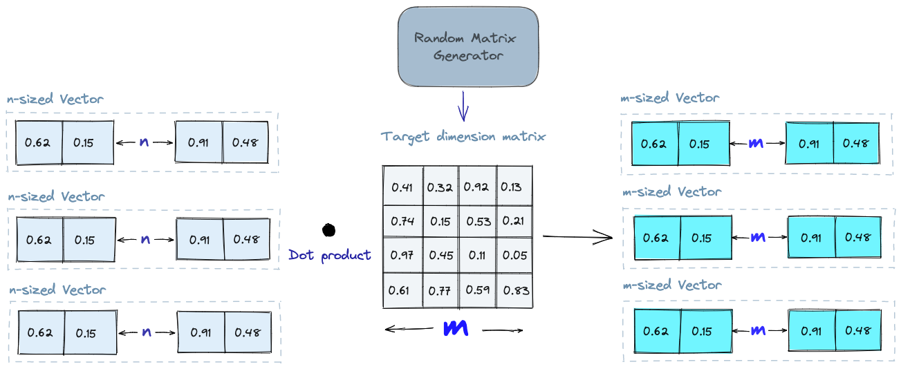
When we query, we use the same projection matrix to project the query vector onto the lower-dimensional space. Then, we compare the projected query vector to the projected vectors in the database to find the nearest neighbors. Since the dimensionality of the data is reduced, the search process is significantly faster than searching the entire high-dimensional space.
Just keep in mind that random projection is an approximate method, and the projection quality depends on the properties of the projection matrix. In general, the more random the projection matrix is, the better the quality of the projection will be. But generating a truly random projection matrix can be computationally expensive, especially for large datasets. Learn more about random projection.
Product Quantization
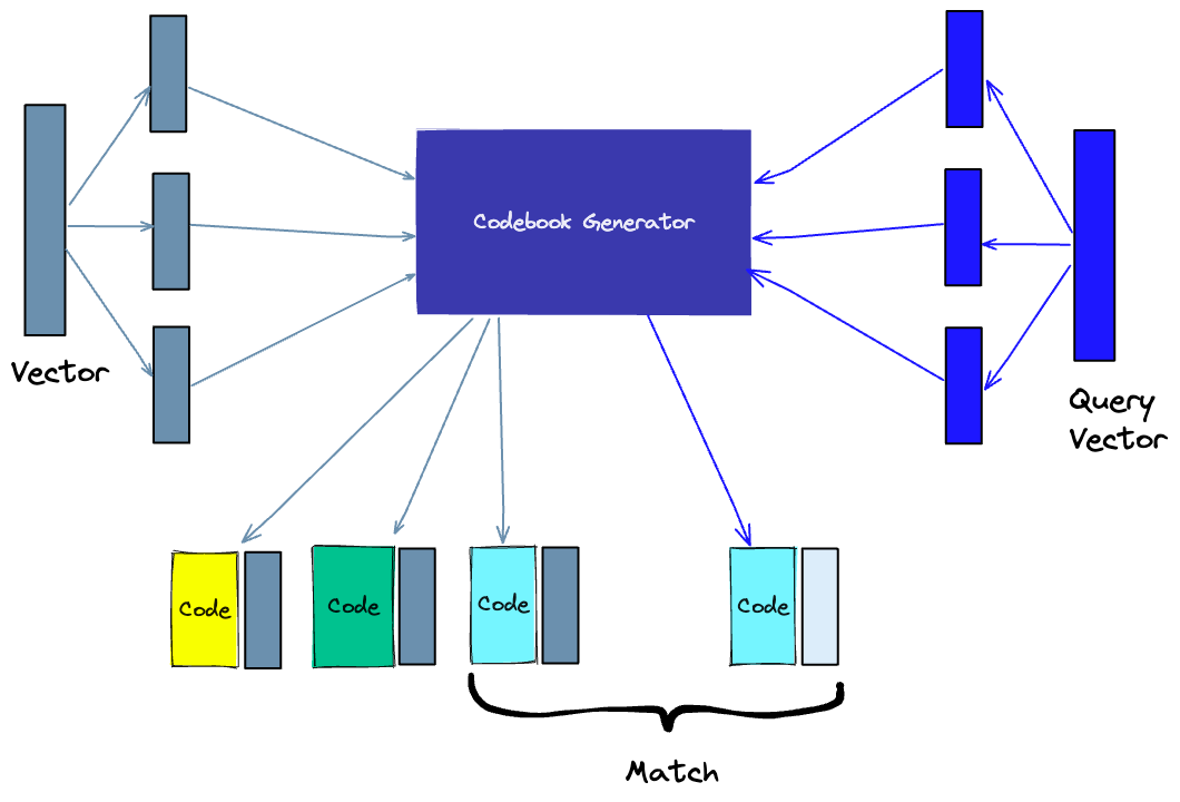
Another way to build an index is product quantization (PQ), which is a lossy compression technique for high-dimensional vectors (like vector embeddings). It takes the original vector, breaks it up into smaller chunks, simplifies the representation of each chunk by creating a representative “code” for each chunk, and then puts all the chunks back together - without losing information that is vital for similarity operations. The process of PQ can be broken down into four steps: splitting, training, encoding, and querying.
-
Splitting: The vectors are broken into segments.
-
Training: We build a “codebook” for each segment. Simply put - the algorithm generates a pool of potential “codes” that could be assigned to a vector. In practice - this “codebook” is made up of the center points of clusters created by performing k-means clustering on each of the vector’s segments. We would have the same number of values in the segment codebook as the value we use for the k-means clustering.
-
Encoding: The algorithm assigns a specific code to each segment. In practice, we find the nearest value in the codebook to each vector segment after the training is complete. Our PQ code for the segment will be the identifier for the corresponding value in the codebook. We could use as many PQ codes as we’d like, meaning we can pick multiple values from the codebook to represent each segment.
-
Querying: When we query, the algorithm breaks down the vectors into sub-vectors and quantizes them using the same codebook. Then, it uses the indexed codes to find the nearest vectors to the query vector.
The number of representative vectors in the codebook is a trade-off between the accuracy of the representation and the computational cost of searching the codebook. The more representative vectors in the codebook, the more accurate the representation of the vectors in the subspace, but the higher the computational cost to search the codebook. By contrast, the fewer representative vectors in the codebook, the less accurate the representation, but the lower the computational cost. Learn more about PQ.
Locality-Sensitive Hashing
Locality-Sensitive Hashing (LSH) is a technique for indexing in the context of an approximate nearest-neighbor search. It is optimized for speed while still delivering an approximate, non-exhaustive result. LSH maps similar vectors into “buckets” using a set of hashing functions, as seen below:
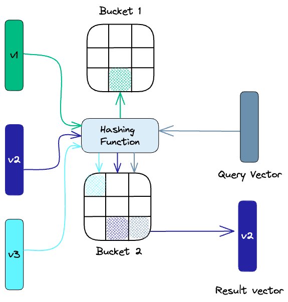
To find the nearest neighbors for a given query vector, we use the same hashing functions used to “bucket” similar vectors into hash tables. The query vector is hashed to a particular table and then compared with the other vectors in that same table to find the closest matches. This method is much faster than searching through the entire dataset because there are far fewer vectors in each hash table than in the whole space.
It’s important to remember that LSH is an approximate method, and the quality of the approximation depends on the properties of the hash functions. In general, the more hash functions used, the better the approximation quality will be. However, using a large number of hash functions can be computationally expensive and may not be feasible for large datasets. Learn more about LSH.
Hierarchical Navigable Small World (HNSW)
HNSW creates a hierarchical, tree-like structure where each node of the tree represents a set of vectors. The edges between the nodes represent the similarity between the vectors. The algorithm starts by creating a set of nodes, each with a small number of vectors. This could be done randomly or by clustering the vectors with algorithms like k-means, where each cluster becomes a node.
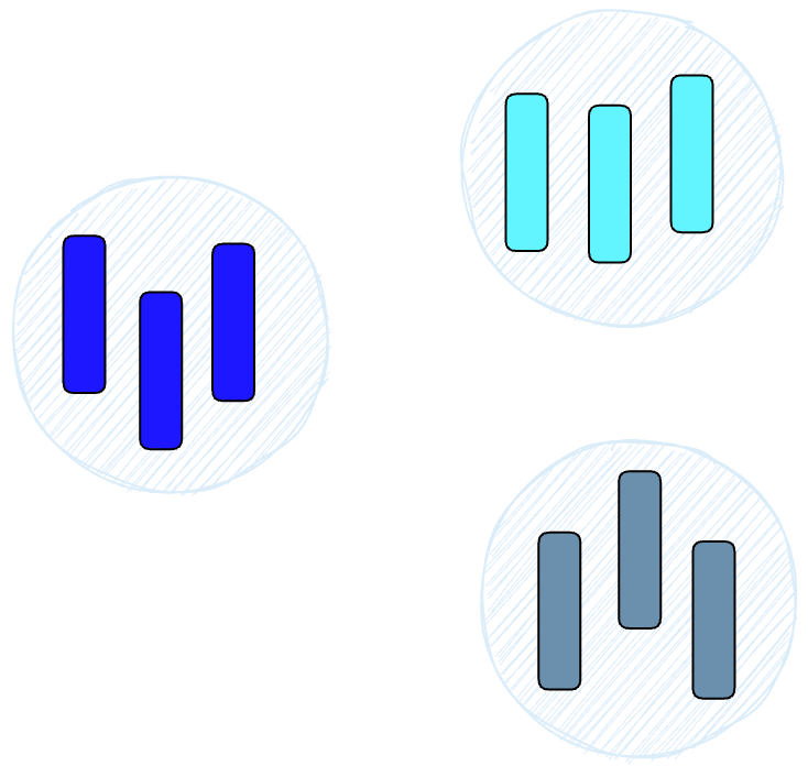
The algorithm then examines the vectors of each node and draws an edge between that node and the nodes that have the most similar vectors to the one it has.h
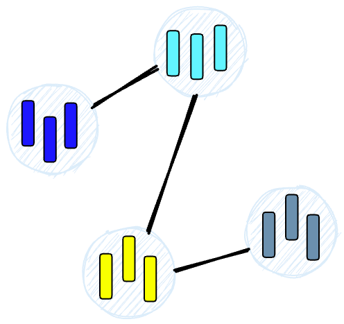
When we query an HNSW index, it uses this graph to navigate through the tree, visiting the nodes that are most likely to contain the closest vectors to the query vector. Learn more about HNSW.
Similarity Measures
Building on the previously discussed algorithms, we need to understand the role of similarity measures in vector databases. These measures are the foundation of how a vector database compares and identifies the most relevant results for a given query.
Similarity measures are mathematical methods for determining how similar two vectors are in a vector space. Similarity measures are used in vector databases to compare the vectors stored in the database and find the ones that are most similar to a given query vector.
Several similarity measures can be used, including:
-
Cosine similarity: measures the cosine of the angle between two vectors in a vector space. It ranges from -1 to 1, where 1 represents identical vectors, 0 represents orthogonal vectors, and -1 represents vectors that are diametrically opposed.
-
Euclidean distance: measures the straight-line distance between two vectors in a vector space. It ranges from 0 to infinity, where 0 represents identical vectors, and larger values represent increasingly dissimilar vectors.
-
Dot product: measures the product of the magnitudes of two vectors and the cosine of the angle between them. It ranges from -∞ to ∞, where a positive value represents vectors that point in the same direction, 0 represents orthogonal vectors, and a negative value represents vectors that point in opposite directions.
The choice of similarity measure will have an effect on the results obtained from a vector database. It is also important to note that each similarity measure has its own advantages and disadvantages, and it is important to choose the right one depending on the use case and requirements. Learn more about similarity measures.
Filtering
Every vector stored in the database also includes metadata. In addition to the ability to query for similar vectors, vector databases can also filter the results based on a metadata query. To do this, the vector database usually maintains two indexes: a vector index and a metadata index. It then performs the metadata filtering either before or after the vector search itself, but in either case, there are difficulties that cause the query process to slow down.
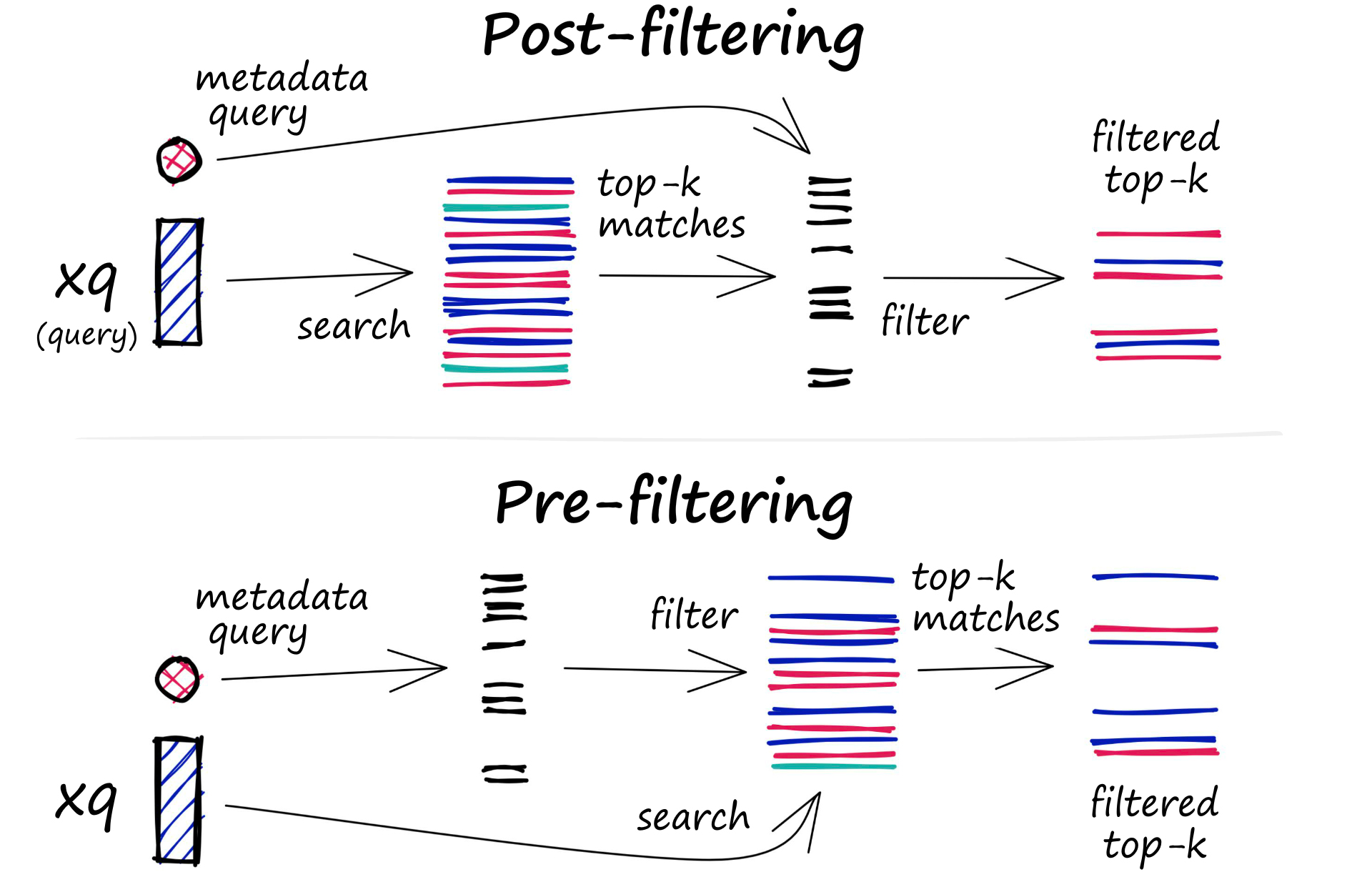
The filtering process can be performed either before or after the vector search itself, but each approach has its own challenges that may impact the query performance:
-
Pre-filtering: In this approach, metadata filtering is done before the vector search. While this can help reduce the search space, it may also cause the system to overlook relevant results that don’t match the metadata filter criteria. Additionally, extensive metadata filtering may slow down the query process due to the added computational overhead.
-
Post-filtering: In this approach, the metadata filtering is done after the vector search. This can help ensure that all relevant results are considered, but it may also introduce additional overhead and slow down the query process as irrelevant results need to be filtered out after the search is complete.
To optimize the filtering process, vector databases use various techniques, such as leveraging advanced indexing methods for metadata or using parallel processing to speed up the filtering tasks. Balancing the trade-offs between search performance and filtering accuracy is essential for providing efficient and relevant query results in vector databases. Learn more about vector search filtering.
Database Operations
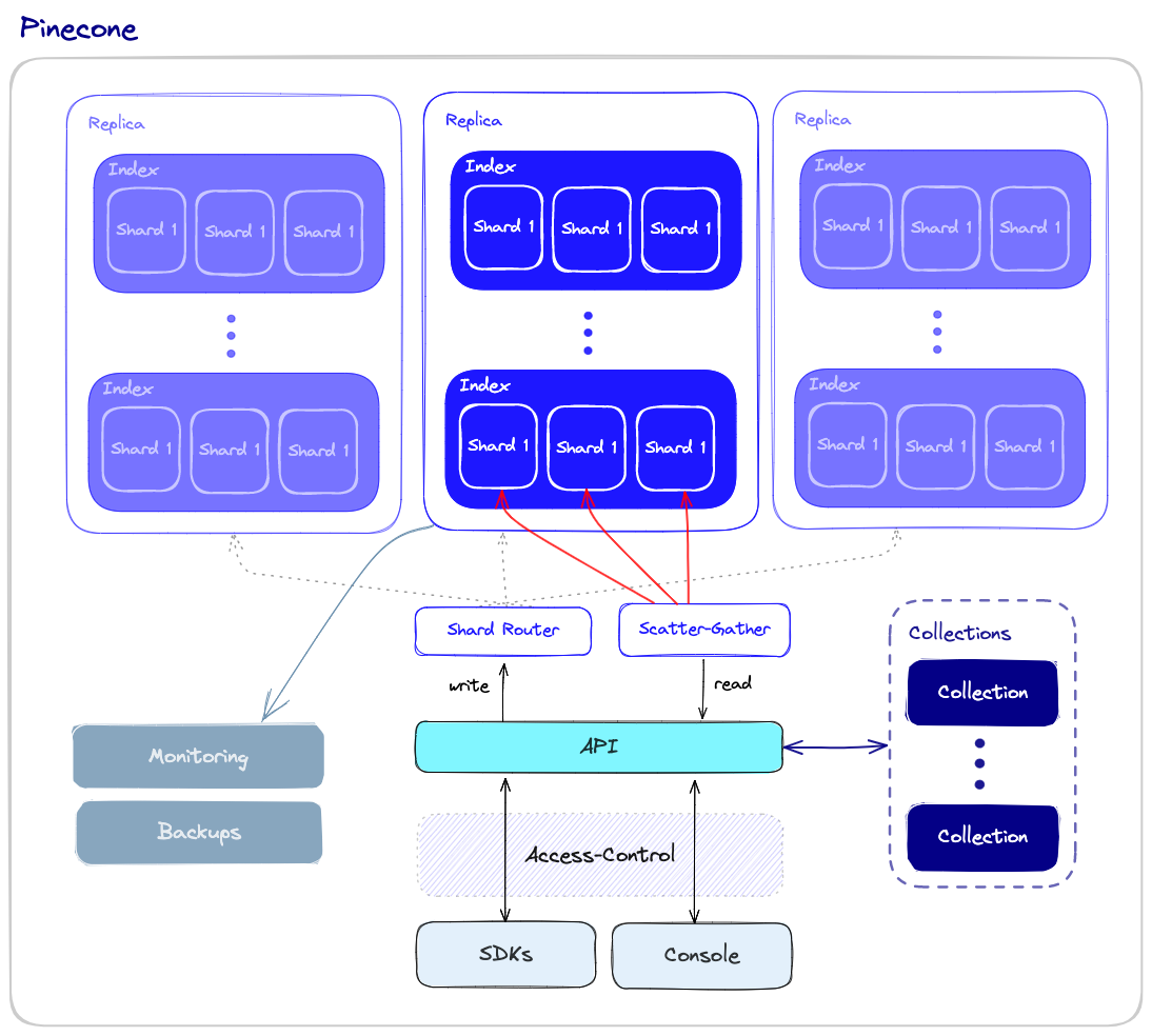
Unlike vector indexes, vector databases are equipped with a set of capabilities that makes them better qualified to be used in high scale production settings. Let’s take a look at an overall overview of the components that are involved in operating the database.
Performance and Fault Tolerance
Performance and fault tolerance are tightly related. The more data we have, the more nodes that are required - and the bigger chance for errors and failures. As is the case with other types of databases, we want to ensure that queries are executed as quickly as possible even if some of the underlying nodes fail. This could be due to hardware failures, network failures, or other types of technical bugs. This kind of failure could result in downtime or even incorrect query results.
To ensure both high performance and fault tolerance, vector databases use sharding and replication apply the following:
-
Sharding - partitioning the data across multiple nodes. There are different methods for partitioning the data - for example, it can be partitioned by the similarity of different clusters of data so that similar vectors are stored in the same partition. When a query is made, it is sent to all the shards and the results are retrieved and combined. This is called the “scatter-gather” pattern.
-
Replication - creating multiple copies of the data across different nodes. This ensures that even if a particular node fails, other nodes will be able to replace it. There are two main consistency models: eventual consistency and strong consistency. Eventual consistency allows for temporary inconsistencies between different copies of the data which will improve availability and reduce latency but may result in conflicts and even data loss. On the other hand, strong consistency requires that all copies of the data are updated before a write operation is considered complete. This approach provides stronger consistency but may result in higher latency.
Monitoring
To effectively manage and maintain a vector database, we need a robust monitoring system that tracks the important aspects of the database’s performance, health, and overall status. Monitoring is critical for detecting potential problems, optimizing performance, and ensuring smooth production operations. Some aspects of monitoring a vector database include the following:
-
Resource usage - monitoring resource usage, such as CPU, memory, disk space, and network activity, enables the identification of potential issues or resource constraints that could affect the performance of the database.
-
Query performance - query latency, throughput, and error rates may indicate potential systemic issues that need to be addressed.
-
System health - overall system health monitoring includes the status of individual nodes, the replication process, and other critical components.
Access-Control
Access control is the process of managing and regulating user access to data and resources. It is a vital component of data security, ensuring that only authorized users have the ability to view, modify, or interact with sensitive data stored within the vector database.
Access control is important for several reasons:
-
Data protection: As AI applications often deal with sensitive and confidential information, implementing strict access control mechanisms helps safeguard data from unauthorized access and potential breaches.
-
Compliance: Many industries, such as healthcare and finance, are subject to strict data privacy regulations. Implementing proper access control helps organizations comply with these regulations, protecting them from legal and financial repercussions.
-
Accountability and auditing: Access control mechanisms enable organizations to maintain a record of user activities within the vector database. This information is crucial for auditing purposes, and when security breaches happen, it helps trace back any unauthorized access or modifications.
-
Scalability and flexibility: As organizations grow and evolve, their access control needs may change. A robust access control system allows for seamless modification and expansion of user permissions, ensuring that data security remains intact throughout the organization’s growth.
Backups and Collections
When all else fails, vector databases offer the ability to rely on regularly created backups. These backups can be stored on external storage systems or cloud-based storage services, ensuring the safety and recoverability of the data. In case of data loss or corruption, these backups can be used to restore the database to a previous state, minimizing downtime and impact on the overall system. With Pinecone, users can choose to back up specific indexes as well and save them as “collections,” which can later be used to populate new indexes.
API and SDKs
This is where the rubber meets the road: Developers who interact with the database want to do so with an easy-to-use API, using a toolset that is familiar and comfortable. By providing a user-friendly interface, the vector database API layer simplifies the development of high-performance vector search applications.
In addition to the API, vector databases would often provide programming language specific SDKs that wrap the API. The SDKs make it even easier for developers to interact with the database in their applications. This allows developers to concentrate on their specific use cases, such as semantic text search, generative question-answering, hybrid search, image similarity search, or product recommendations, without having to worry about the underlying infrastructure complexities.
Conclusion
The exponential growth of vector embeddings in fields such as NLP, computer vision, and other AI applications has resulted in the emergence of vector databases as the computation engine that allows us to interact effectively with vector embeddings in our applications.
Vector databases are purpose-built databases that are specialized to tackle the problems that arise when managing vector embeddings in production scenarios. For that reason, they offer significant advantages over traditional scalar-based databases and standalone vector indexes.
In this post, we reviewed the key aspects of a vector database, including how it works, what algorithms it uses, and the additional features that make it operationally ready for production scenarios. We hope this helps you understand the inner workings of vector databases.
